Wake effects
What are Wake effects?
When placed within a farm, wind turbines produce disturbances to the air as they extract kinetic energy. These disturbances are commonly referred to as wakes.
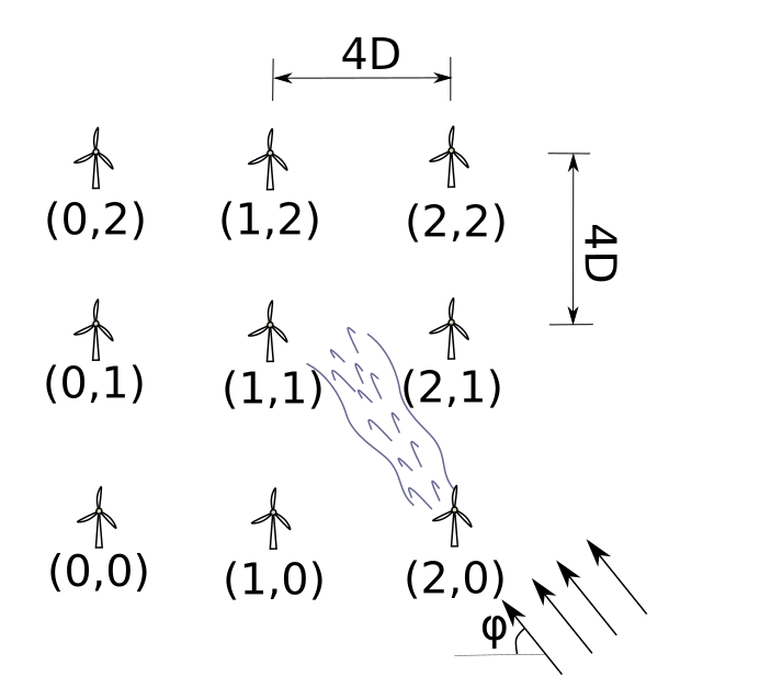
Due to the complex aero-dynamic interactions, wakes may affect turbines that lie downwind in a non-obvious manner while evolving on real wind farms. Moreover, different ambient wind conditions, such as turbulence and temperature, affect how wakes develop. Wakes dramatically affect the power production of wind farms, making the minimum spacing of wind turbines an important design constraint. In order to obtain reliable estimates on power production, and potentially to structural dynamic loads of wind turbine components, it is important to have an automated and scalable technique to model the effect of wakes under different wind conditions statistically.
This work is based on a Monte-Carlo simulation of a windfarm, containing 1000 cases with different wind turbulence intensity, wind orientation, and mean windspeed conditions using NREL-OpenFAST [1] and the Dynamic Wake Meandering subroutines [2]. Each simulation required approximately 13 hours to complete. The volume of the data was too large to post-process in a single machine. Therefore a fully distributed workflow (simulation and post-processing) was implemented in ETH cluster Euler (IBM spectrum LSF system). This also led to my first small contribution on an open-source project, which was to refactor parts of the source code of NREL-OpenFAST to compile and run under Linux. In our related work , presented at the IMAC XXXVI conference , it was demonstrated how deep generative models, namely the Variational Autoencoder (VAE)[3] can effectively represent the statistics of the effect of wakes on the operational characteristics of a wind farm, with a limited amount of samples considering the dimensionality of the problem.
The loss function of the VAE reads:
\[ELBO(X,z) = E[\log P(X \vert z)] - D_{KL}[Q(z \vert X) \Vert P(z)]\]Where \(X\) are the raw monitoring variables, \(z\) is a lower-dimensional representation of the raw variables.
The loss function of the VAE attempts to jointly discover a lower-dimensional representation for the data and warp the raw data in such a way that it is modeled with a simple probability distribution. The \(D_{KL}\) term pushes the lower-dimensional representation \(z\) to a simple probability distribution, whereas the second term helps is forcing the identification of the latent structure in the data.
More specifically, a conditional VAE is used, which is better described in my other post, where I applied this to simulated fatigue loads of wind turbine blades.
Some Results
In the following animation, samples from the trained autoencoder are shown, where the mean wind speed of the farm is controlled. The arrows represent the wind orientation as it is sensed from each turbine.
Effective turbulence intensity is another parameter affected by the wakes.
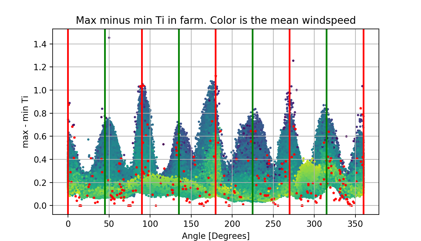 Red dots correspond to the simulated cases. The rest of the data points correspond to samples from the VAE, which generalizes realistically from the available data.
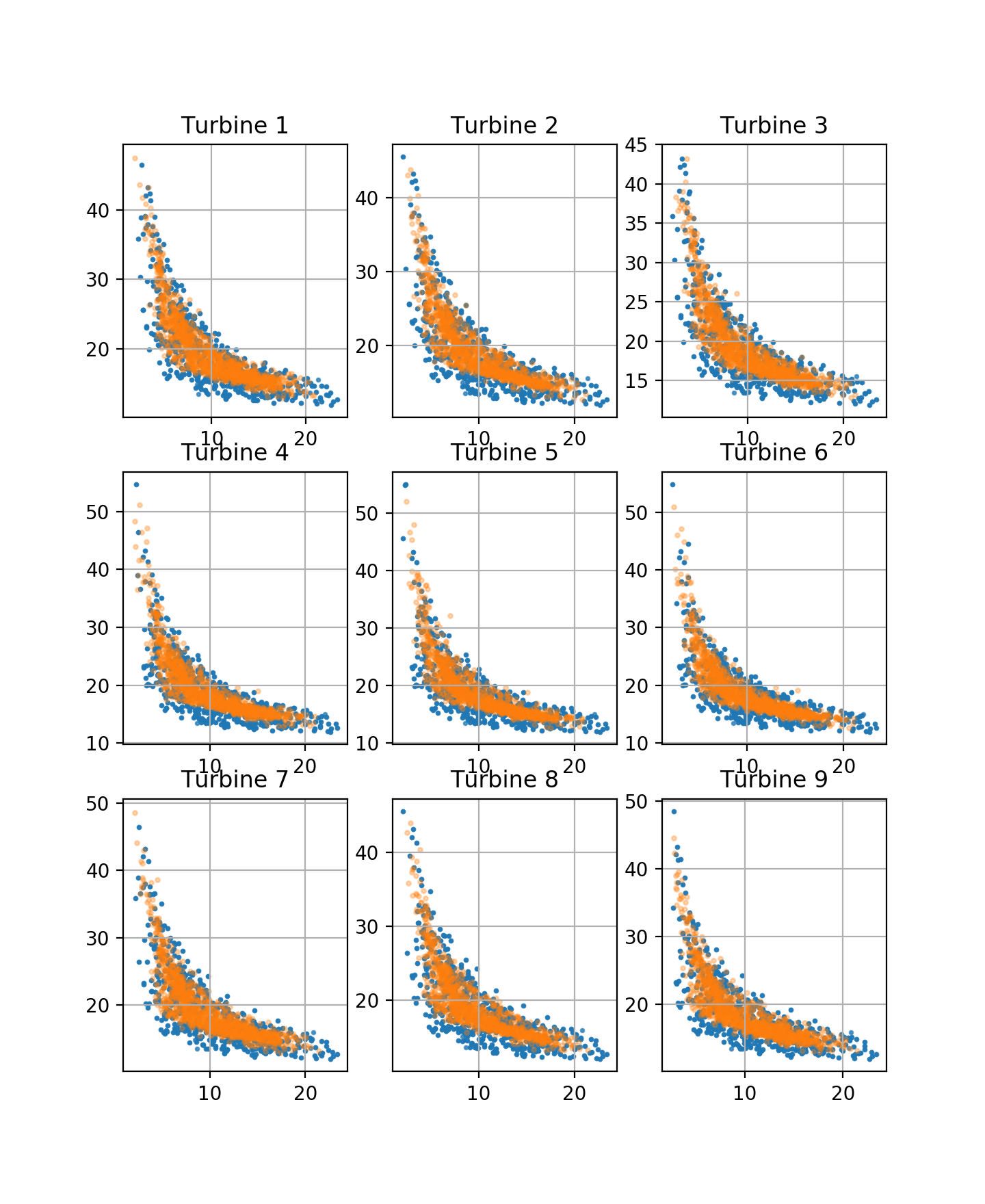 The orange dots correspond to VAE-sampled data, whereas the blue corresponds to data from the test set.
The VAE effectively captures the joint distribution of the wind characteristics at different points, accounting for the effect of wakes.
The orange dots correspond to VAE-sampled data, whereas the blue corresponds to data from the test set.
The VAE effectively captures the joint distribution of the wind characteristics at different points, accounting for the effect of wakes.