The project

Wind turbine fatigue estimation relies on running computationally expensive simulations. The inputs of the simulations (the Windfield time-series) are non-deterministic: We have statistical models on how the wind behaves under different conditions, and we simulate these inputs before applying them to the turbine. Also, the complex dynamics (blade geometric non-linearity, pitch control, etc.) make the response even more difficult to approximate with an explicit model. Finally, in order to make the most out of our simulations, we need to analyze fatigue on the cross-section/material level, and not simply on some so-called hot-spot locations, or manually decompose the damage on some intuitive basis. For example, the standard practice in wind turbine blades is analyzing bending directions separately.

This project was about training a VAE to sample from expensive fatigue simulation outputs. The fatigue is computed with the dynamics simulation/cycle counting procedure, which is typical for wind turbine design and structural analysis.

Engineering application/motivation

There are several applications where this fast sampling procedure becomes relevant in wind energy engineering. This post focuses on one potential real-life application. Consider that one has only historical summary statistics on the weather. The summary statistics collected from the turbine, which typically include the hub-height wind-speed statistics, are going to be referred to as Supervision Control and Data Acquisition systems (SCADA) data. It is not possible to completely reproduce the stress states on the structure because they were never sensed and stored. This situation is close to what is often referred to as “aleatory” uncertainty - the uncertainty that is due to purely random effects and is irreducible. The indeterminacy involved in the problem of fatigue load analysis from SCADA data is closer to “ambiguity” rather than “uncertainty,” but the concept of aleatory uncertainty is closer to the problem at hand. Consider a way to sample a wind field that resembles statistically one that produces summary statistics (like the ones we have available in the SCADA data) already exists. The wind field is typically modeled with some rather empirical models of turbulence.

Short side-note:

The CVAE (or other generative models) would be an excellent fit for the problem of statistically modeling wind as well. I later discovered publications doing exactly that with another type of generative model (the so-called continuous-time normalizing flow withNeural ODE that relies on invertible transformations).

In order to have a robust estimate on accumulated fatigue damage, one would need to run the simulation several times for each SCADA reading, say 100 times (an estimate on the low side). So in order to perform damage accumulation for 10 minutes for one turbine, we would need 100 * 1h = 100h worth of simulation time. This is only for 1 SCADA reading. Obviously, this is not a scalable approach. Focus is shifted to a technique that can work on the millisecond scale instead of the one-hour scale to perform long-term fatigue calculations.

The variation of fatigue estimates is not due to “noise” but due to the incomplete knowledge of the loading conditions in the cross-section. Therefore it is not correct to average them out. The effect of the un-observed dynamics acts as a hidden (latent) factor influencing the actual fatigue distribution. The goal is to create a model that can sample the hidden effect, which we cannot determine from the coarse SCADA observations, and at the same time condition the sampling according to observed factors which we know that potentially influence the fatigue distribution. Moreover, there is no PDE or physical law describing the distribution of fatigue on a wind turbine cross-section, and coarse empirical approaches on the interpretation of simulation outputs of fatigue exist (e.g., the decomposition of fatigue in flap-wise and edge-wise fatigue). A technique that would not need to make such coarse simplification compromises is needed. An appropriate model for this task is a Conditional Variational Autoencoder (CVAE).

The architecture of the CVAE looks as follows during training:

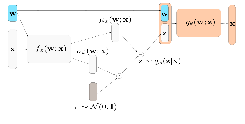
Where w is the “conditioning” inputs and x is the fatigue loads of the cross-section. One cross-section of the the blade is visualized partially because visualization is easier with this geometry. In the present case, w is a vector of SCADA data: wind, turbulence, and a parametrization of the wind velocity distribution along with the height of the wind turbine.

Training dataset and tricks

The training dataset contained fatigue estimates for 2000 randomly sampled SCADA conditions on 250 finite elements. Models with varying sizes were trained to employ some techniques to allow for more reliable convergence (e.g., KL-annealing, burn-in of the KL term, etc.). Extensive hyperparameter sweeps were performed while manually observing samples from the CVAE and random samples of batches of nearest neighbors for the same latent from the testing set. Relatively small models were trained. For instance, results from a feed-forward model with (affine)/(relu 50)/(relu 50)/(linear 25/softplus 25) - latent 15 - (relu 50)/(relu 50)/(relu 50)/(linear) decoder are shown in what follows. The main mode of fatigue damage (bending due to self-weight of the blade, in tandem with pitch variations) on the cross-section is expected and easily interpretable due to physical reasons. (update: In retrospect, even smaller models, less deep models, could have worked well. The latest work from Nvidia (NVAE paper seems to suggest that for more powerful models in the VAE framework, hierarchical latent variables as in ladder VAE and some further computational tricks are important. ) Through extensive experimentation, it seems that the latent space size was not critical for this problem. The latent space is not necessarily interpretable in the present problem. The objective related to the use of VAE in this problem is not to obtain an interpretable latent space in the first place. The goal is to quantify the uncertainty in estimates of fatigue, given only 10-minute SCADA data information and without making assumptions on their spatial distribution.

In the way this problem is posed, it is important that there is little to no “structure.” in the latent space. When “structure” in the approximate posterior \(\mathcal{N}(\mathbf{z}|\mu(\mathbf{x}),\mu(\mathbf{w}))\) exists, we cannot safely replace the approximate posterior with a diagonal Gaussian. In that case, approximating with a Gaussian will allow sampling from regions of the latent space that decode to completely unrealistic points in the physical space. A recent paper refers to this as the “holes” problem of VAEs (paper: Taming VAEs).

After training the model, one may simply discard all the “light gray” parts of the previous figure (the “encoder”), sample z from a unit Gaussian, and include the conditioning variables on the decoder part. Follows a visualization of samples of accumulated damage equivalent loads from the CVAE, with one actual realization for the time window for two cases:

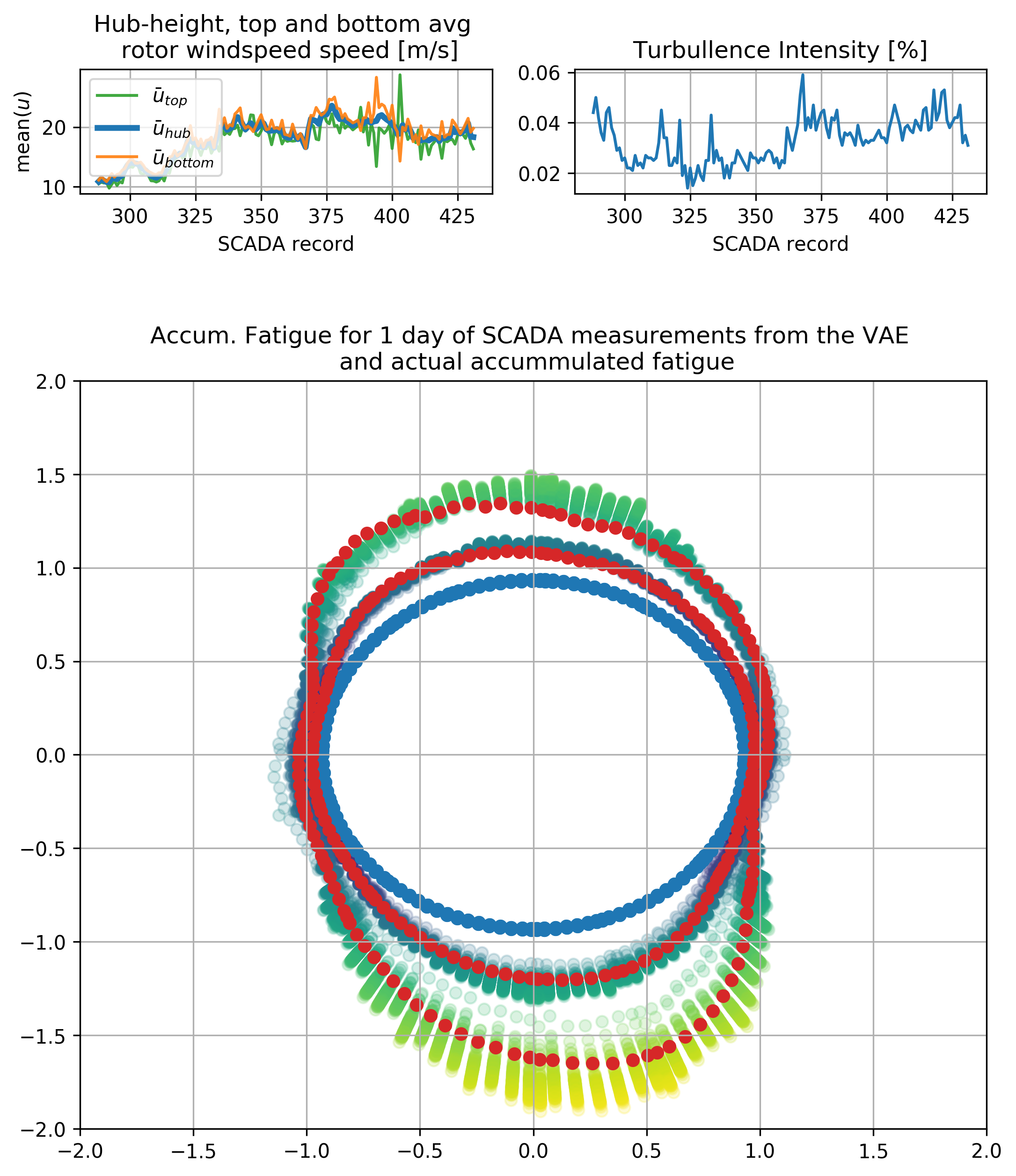
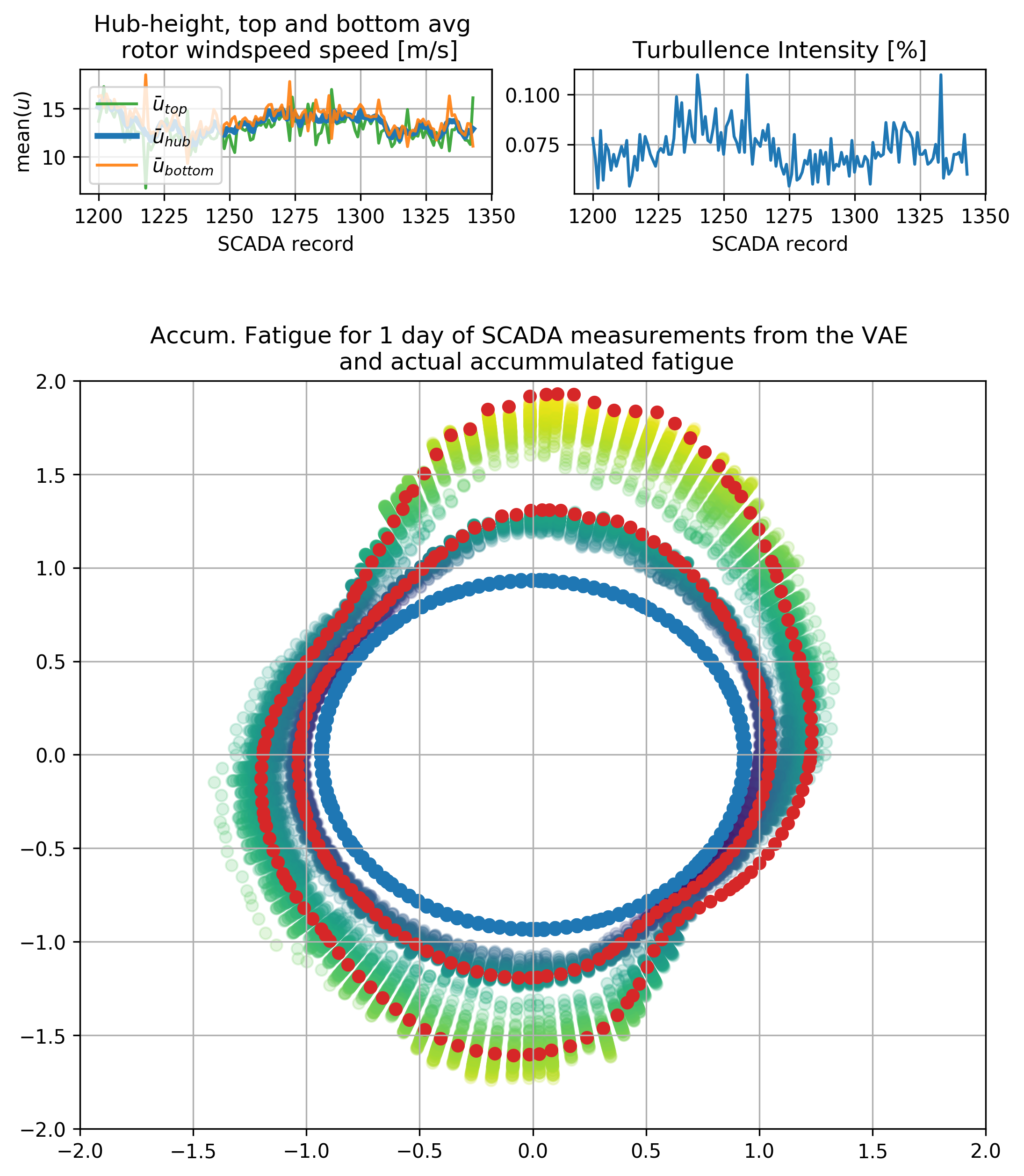
Notice the highly non-linear dependency on the inputs. Also the VAE returns results for the whole cross-section and not only for single points.

Conditional variational autoencoders - animation

This application used a Conditional VAE since we know beforehand the influencing factors we care about. It is possible to interpolate the input variables and inspect their effect on the output. The latent space does have an effect and it is seen on the previous plots. Namely, this effect is observed in the variability on the sampled estimates of damage equivalent loads.

Thank you for reading! Check out the recently published (Feb. 2021) paper here. You can find a tensorflow 2.4 + tensorflow probability implementation of the CVAE in (github.com/mylonasc/fatigue-cvae).